Chapter 18 Extensions to Supply and Demand
Price elasticity of demand mid-point formula:
Numerator is change in quantity ___________________________ 0.5(Q1 + Q2) Denominator is change in price ___________________________ 0.5(P1 + P2) Class presentation: 1. Price elasticity of supply formula and what price elasticity of supply means 2. Price elasticity over market period, short run, long run 3. Price elasticity applications 4. Cross elasticity of demand formula and what cross elasticity of demand means 5. Substitutes, complementary goods, and independent goods using cross elasticity of demand 6. Income elasticity of demand formula and what income elasticity of demand means. Normal and inferior goods and expansion of the economy using income elasticity of demand 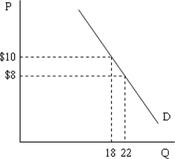
Practice
|
Chapter 19 Consumer Behavior and Utility Maximization
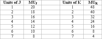
Refer to the above table. If this consumer has an income of $26 and the prices of J and K are $2 and $4 respectively, the consumer will maximize her utility by purchasing:
A)7 units of J and 3 units of K B)5 units of J and 4 units of K C)3 units of J and 5 units of K D)1 units of J and 6 units of K Divide each of the entries in the MUJ column by $2 and each of the entries in the MUK column by $4 to obtain the marginal utilities in terms of per dollar spent on each good. The first dollar will be spent on K because it provides 12 units of utility, whereas J would provide only 10 units of utility. Continue in this manner, purchasing the next unit of the good with the highest marginal utility per dollar until income is exhausted. At this point, the marginal utility per dollar of each good will be the same—6 units of utility per dollar in this example. (B) Jim enjoys having either a peanut butter sandwich or a bologna sandwich for his lunch. A drop in the price of peanut butter increases the marginal utility per dollar of peanut butter and causes Jim to buy more peanut butter and less bologna to restore maximum utility. This best illustrates the: A)law of diminishing marginal utility B)income effect C)substitution effect D)law of increasing total utility The substitution effect of a price decrease refers to the impact on quantity demanded because this good is now relatively less expensive compared to its substitutes. | ||||||||
Chapter 21 Perfect (Pure) Competition
Practice tests and more here and here.
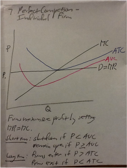
The individual firm will view its demand as perfectly elastic. A perfectly elastic demand curve is a horizontal line at the price. The demand curve for the industry is not perfectly elastic, it only appears that way to the individual firms, since they must take the market price no matter what quantity they produce. Therefore, the firm’s demand curve is a horizontal line at the market price. Marginal revenue (MR) is the increase in total revenue resulting from a one-unit increase in output. Since the price is constant in the perfect competition. The increase in total revenue from producing 1 extra unit will equal to the price. Therefore, P= MR in perfect competition. Overview video here. Firm v market here.
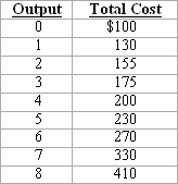
Refer to the above data for a competitive market. If the market price is $35 and the firm produces its optimal amount, it will realize how much profit or loss?
To find the optimal output level, use the cost data to determine marginal cost. The marginal cost of the fifth unit is $30 and the marginal cost of the sixth unit is $40, so producing five units is optimal. Total revenue is $35 times 5 units, or $175. Since the total cost of five units is $230, the firm incurs a loss of $55. Note that cost is $100 when output is zero, so incurring a $55 loss is better than shutting down and incurring a loss of $100. 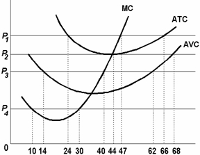
|
Chapter 20 The Costs of Production
Practice tests and more here
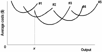
The diagram shows the short-run average total cost curves for five different plant sizes for a firm. The firm experiences economies of scale over the range of plant sizes: 1 through 3 only. If a firm is experiencing economies of scale, its short-run average total cost curves will be falling. More on explicit versus implicit costs here. More on costs of production here and video here. Student cost analysis of a restaurant below:
| ||||||||||||||||||
| _apeconch21study_guide-1.docx |
Chapter 22 Pure Monopoly
Practice tests and more here.
|
Chapter 23 Monopolistic Competition and Oligopoly
Monopolistic competition overview here. Game theory here, here and here. Nash equilibrium here and here. Practice tests and more here and especially here or here. Size and innovation here. Kinked demand curve here.
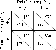
Refer to the matrix, which shows the profit payoffs to each of two oligopolistic firms of following either a high- or low-price policy. Gamma's payoffs are in the lower left corner of each cell; Delta's in the upper right. If Gamma uses a high-price strategy and Delta uses a low-price strategy what will Gamma want to do next?
Given the assumed strategies, Gamma's profits are $20 and Delta's profits are $75. Given Delta's strategy, Gamma's profits would increase to $30 if it switched to a low-price strategy. Extra Credit: You may earn either two or six points extra credit. However, if 10% or more of the class picks the six-point option, no student earns extra credit. Extra credit: Respond to this article with a logical response, agreeing or disagreeing with the author's conclusions. | ||||||||||||||||||||||
|
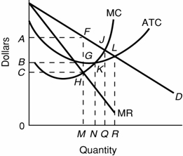
If this firm produces its profit-maximizing output, its potential profit is:
Maximum profits are earned by producing M units and selling them at price A. The firm earns a profit of $(A – G) on each unit—the difference between price and average total cost. Total profit is this amount per unit for each of the M units sold, for a total of area AFGB. |
